Neural Networks

Overview

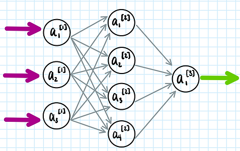
Neural networks are a form of supervised learning. They learn from labeled data how the data groups can be optimally identified (classified). The algorithm is modeled after biological neural networks in the brain. It is constructed from basic units ("neurons") which each consist of a linear component and an activation function (Figure 65). The linear component of the neuron takes the form W*x + b, where x is an array of the inputs to the neuron, W is an array with the weights for those inputs, and b is an array with biases. W and b are tunable parameters of the network. The result of the linear component then passes through the activation function of the neuron, such as a sigmoid function. This transformed result is then passed to other neurons, deeper into the network. Neurons are organized into "layers," and layers of neurons are interconnected with each other (Figure 66).

When the model trains on a subset of data, the network parameters (weights and biases) are updated iteratively. At each training iteration (epoch), the output of the network (prediction) is compared to the training label (ground truth). The error (difference) is then used to tune the network parameters (i.e., "back propagation").

Figure 65: Top- example with biological neurons. The neuron in black receives signals from three neurons (purple) as input. The strength of the connections (synapses) between the different purple neurons and the black neuron may vary. If the black neuron receives sufficient input to surpass it's activation threshold, it "fires" (produces an output, green). Bottom- same example with artificial neurons. Here, the inputs to the black neuron are represented by the vector X, and the strengths of the different synapses are represented by the weights vector, W. The inputs are summed linearly and then sent to the activation function, which in this case is the sigmoid function.

Figure 66: Example diagram of a neural network model. Neurons are represented by black circles and denoted by the letter a. The superscript represents the layer of the neuron within the network, and the subscript identifies the neuron within each layer. Input to the model is sent to the first layer (superscript 1). This is also called the input layer. These neurons are fully connected with those of the second layer (superscript 2). This second layer is referred to as a "hidden" layer, since it is hidden from both the direct input and direct output. A network may have multiple hidden layers, but this example has only one. The hidden layer then connects to the third and final layer (superscript 3), which produces the output of the model ("output layer").

Data Preparation

LINK TO SAMPLE OF THE DATA

LINK TO CODE

For a preview image of the raw data/starting point, please see FIGURE 16 on the Data Prep & Exploration tab of this website.

For this project, we will be using a neural network to attempt to classify whether a song is "preferred" or "not preferred" by a user given a set of attributes from our acquired MSD and Spotify data.

Creating the data labels/classes. The outcome variable for this classification problem will be called "Preferred" and will have a value of 1 for preferred, and 0 for not preferred. We will determine whether or not a song is preferred using the playcount information in our dataset. For each user, their mean playcount (from all of their listened-to songs) is calculated (Figure 67). For a given song which a user listened to, if the song playcount is over their mean playcount, then that song is labeled as "preferred" (1). Alternatively, it is labeled as "not preferred" (0).

Cleaning & balancing the classes in the dataset. After labeling our data, we calculate the playcount variance within each user and remove users with a variance of less than 3. We have a large quantity of data (likely more than what we can realistically use in the algorithm later), so doing this will help retain users with a wider range of playcounts and perhaps help our classification accuracy later. We then check the prevalence of each class in the dataset. In doing this, we find that there's about half as many "preferred" observations as there are "not preferred" observations. This imbalance should be corrected for, as the bias in our dataset will likely also bias our classifier. The data are sampled such that there are an equal number of observations from both classes.

Creating "preference distance" attributes. Before attempting classification, we create two more attributes which may assist with the preference classification task. Please refer back to the Introduction tab for an overview of how this quantitative metric was initially developed and utilized in prior works. In this project, we will be calculating "preference distance" a little differently. In prior works this metric was calculated within the context of the MUSIC five-factor model space. Due to time constraints with this project and the time-consuming nature of accurately translating our data into the MUSIC space, we will do an analogous calculation using some of the Spotify acoustic attributes instead of the MUSIC factors. The following attributes will be used from our dataset:

trackAcoustic: track "acousticness" score.
trackDanceable: track "danceability" score.
trackEnergy: track energy score.
trackInstrum: track "instrumentalness" score.
trackSpeech: track "speechiness" score.
trackVal: track overall valence measure.

I intentionally selected the high-level attributes from our dataset, to more closely parallel the high-level descriptive nature of the MUSIC factors and did not include the loudness or tempo attributes.

For each user, their mean for each of the attributes listed above is calculated (from all their listened-to songs). This gives us a 6-dimensional centroid for each user which can be taken to quantitatively represent their average listening habits on each of these six musical attributes (Figure 67). From there, a "preference distance" is calculated for each of a user's songs by taking the absolute difference of the song's corresponding attribute values and their "centroid." This metric represents how similar a given song is on these six musical attributes to what that user has typically reported listening to. In contrast to previous parts of this project which calculated the preference distance using cosine similarity, resulting in one numeric value, here we will keep the six attributes separate and instead calculate the similarity for each independently. This will result in six numeric values for each user and song, describing the song's similarity to the user's profile. This will allow for the model to have a little more flexibility with the attributes and how they are weighted/combined. As was suggested in the results so far, some of the six attributes may play more of a role in determining preference than others.

Figure 67: A temporary dataframe created to store mean attribute values for each user in our dataset. The mean_playcount variable is calculated from the playcounts for all of a user's songs. Mean playcount will be used later to create our dataset labels. Similarly, the six right-most columns of the dataset represent the mean acoutic attribute value for that user's data. These mean/center values for each user represent their average listening habits (in terms of musical characteristics) and will be used later to calculate the preference distance (similarity) metric.

A preview of the final dataframe is shown below.

Split data into train / test subsets. Because neural networks learn from labeled data, we need to train the model on a subset of labeled data and then test its performance on a separate, previously unseen subset of the data. We will use the common split proportion of 80% of our data for training, and 20% for testing. The rows of the dataframe (shown above) are shuffled/randomized. Then, the first 80% of the rows are saved as the training set, and the last 20% are saved as the testing set. This gives us two disjoint sets / data files. Sets that are not disjoint will misleadingly inflate the performance of the model. The full dataset, as well as the split train/test files can be found here. Figure 68 below shows a preview of the train and test sets.

Figure 68: Training set (top) and testing set (bottom) previews (first five rows of each).

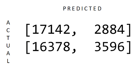
Model performance. The model used a mean squared error loss function. After training for 20 epochs it had a train accuracy of about 50%. The results for the test set are shown below. The test accuracy is 51.85%, which is poor for two classes.

Results

The neural network was implemented using TensorFlow in Python. The structure of the model is illustrated below. The model has three layers, a linear input layer, hidden layer with RELU activation function, and output layer with softmax activation function.

Code is available here.

Conclusions

In this section, we used neural networks to attempt to classify user preferred and not-preferred songs. We experimented with a different representation of the preference distance than in the previous parts of the project. Prediction accuracy overall was incredibly low for a two-class problem. Testing the network with the same data used for the SVM in the previous section still resulted in a very low accuracy. This suggests that the neural network model was not implemented effectively in this section, and the poor performance is not necessarily due to the preference representation used.